In prior articles, we stated the potential economic benefits of measurement and automation of freeness. However, to avoid hyperbolic estimates that overpromise and under-deliver, rigorous analytical techniques exist that can provide reasonable expectations of benefits. Some of those techniques are explained in the references at the end of this article.
Don’t Chase Noise
The fundamental principle is that we should not chase noise. Noise is a random variation at a frequency higher than an actuator can respond to it. Noise can arise from phenomena such as raw material variation (unique attributes of each fiber), mechanical vibration (refiner plate gap that dithers), mechanical imprecision (refiner plate bars that are not uniform), power variation (transmitter power supply), or electromagnetic interference (a motor near a signal that induces variation in the signal). We would all wish for a noiseless process, and there are design solutions that can mitigate them, but it cannot be made perfect and automatic control cannot (and should not) attempt to address noise. Trying to reduce noise through automation will only amplify it.
Therefore, we need to segregate the noise from substantive change. There are two methods for doing this:
- There is a long-standing and time-tested principle known as the Shannon Sampling Theorem. It states, “If a system uniformly samples an analog signal at a rate that exceeds the signal’s highest frequency by at least a factor of two, the original analog signal can be perfectly recovered from the discrete values produced by sampling.” Another way of saying this is that you cannot consider any signal to have significant changes until you have two or more that show that change. If you only have one data point that has significantly changed, you don’t know if it is significant. You could be chasing noise. In practice, you want to filter your raw signal for at least three times the sampling rate. If a moving average filter is used, you will calculate the average of the last three values as your control signal. It is more common to use exponential filters where a time constant can be specified as three times the sampling period. For example, if you are sampling every second, your filter would be configured for a 3-second time constant. If you are familiar with Fourier transforms, this removes the power spectrum below the time constant in your filter. The remaining variation in the power spectrum is what could be addressed with automation.
- There is another practical limitation. A refiner is not to be used as a fast-acting actuator. Instead, changing the gap or specific energy on a refiner should be done gently to address swings or drift in freeness. The time constant for this response differs depending on equipment and the process, but a typical response time for the gap adjustment to settle to a persistent freeness change is about 1 minute. Therefore, the control tuning, in this case, should aim for a closed loop time constant of 1 minute, meaning that a disturbance to freeness should be returned to the desired setpoint in about 1 minute.
1-Second Freeness Sample vs. 5-Minute Freeness Sample
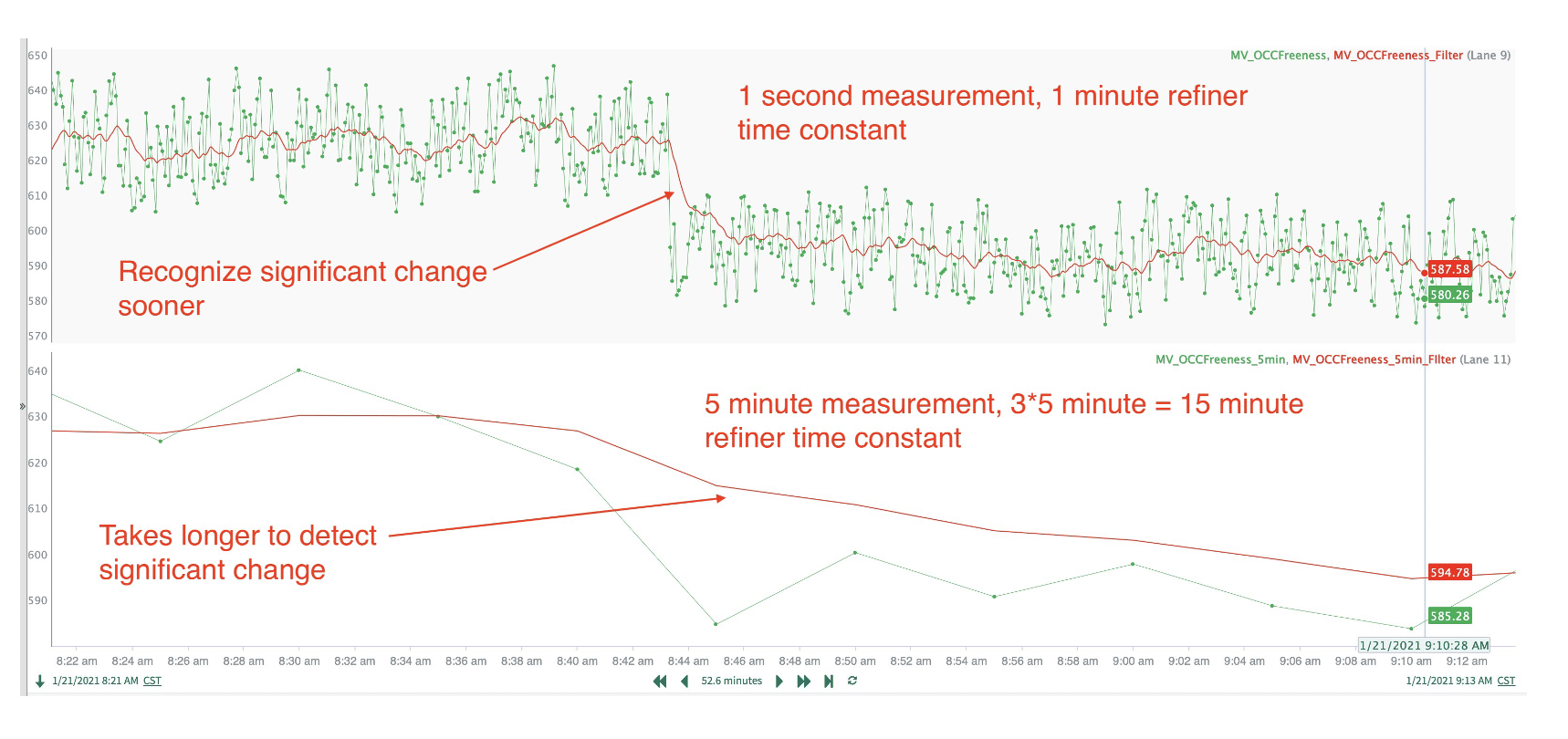
To illustrate these concepts simultaneously, consider a freeness sensor that samples at 1 second compared to another at 5 minutes. The refiner response time is 1 minute. Therefore, for a sensor sampling at 1 minute, the limiting factor is the response of the refiner. We can then use a filtered value with a 1-minute time constant. For the 5-minute measurement, the limiting factor is the Shannon Sampling Theorem, which would impose 3 x 5 minutes – 15-minute time constant for the filter. The results shown below compare these two raw signals and the resulting filtered value to be used for the control input:
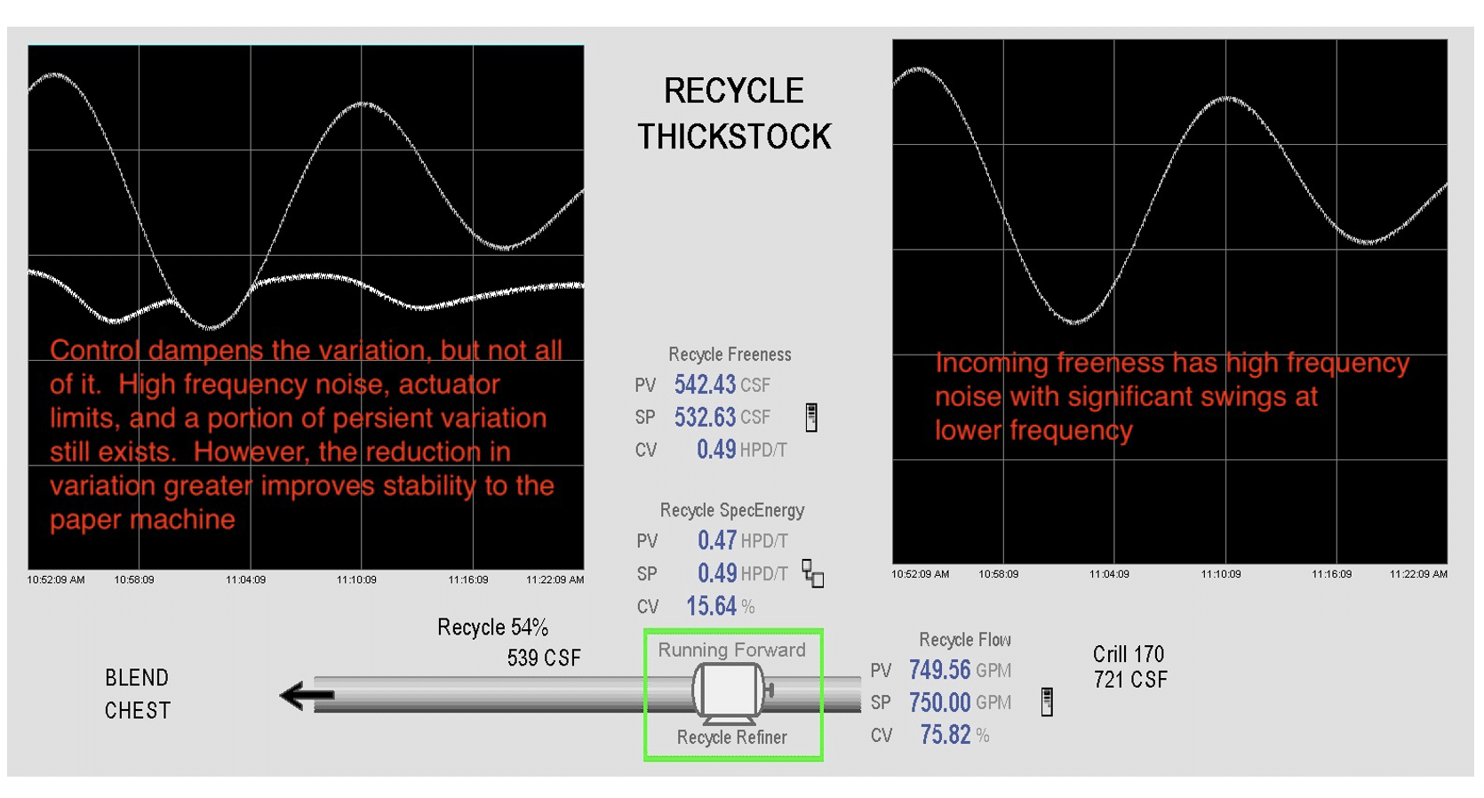
This shows that a freeness change would pass more variation on to the headbox when the sampling frequency is slower, but even at a faster sampling rate, the freeness “noise” would still exist. Therefore, a control loop using a 1-second freeness measurement would likely give the following results:
This can typically account for a 75% reduction in variation, which will reduce breaks, stabilize the dry line, enable faster production, and ensure consistent quality. As stated in the previous article, a typical paper machine could see a $9 million annual benefit from this automation.
The Pulmac Difference – the partner with the holistic knowledge of fibers, papermaking, data analytics, and automation.
The difference between an implementation that delivers these benefits and one that doesn’t is to have a partner that understands fibers, papermaking, data analytics, and automation.
Many automation professionals don’t understand fibers and papermaking and may not have the depth of PID control theory to properly handle nonlinearity and optimal performance.
Pulmac is the industry leader in unlocking the mysteries of fiber properties and now has industry-leading data analytics and automation expertise. This is how these benefits get delivered on day one and beyond. Given the heavy workload of onsite engineers, Pulmac can provide the expertise and resources to deliver this solution promptly and cost-effectively.
Pulmac can assess the benefits of freeness measurement and control for your paper machine using sound and realistic engineering principles. Let us help you with a study of your machine to show you the benefits we can offer.
References:
Analysis of paper machine performance”, Michael F Saucier and Alan D Steinkircher, April 1988, Tappi Journal
Estimating control function benefits”, G.D. Martin, L.E. Turpin, and R.P. Cline, June 1991, Hydrocarbon Processing


